Model Performance

Overview

This section discusses the model performance from the implementation of the different models that served as target pools in DARTS. What follows is a description of the features, followed by an overview of the algorithms applied, discussion of the overall performance results and error analysis.

Description of Features

We used a feature set that included demographics, jurisdictional attributes, socio-economic status, voting history and survey data on people’s attitudes on a variety of political and social issues. We reduced the dimensionality of the feature set for modeling purposes using statistical analysis approaches (correlation analysis and Boruta methods) and intuition around thematically-related features. Features were engineered and normalized to scale for model implementation. The sources of this data included voter profile data and survey response data provided by the People’s Action campaign.

Algorithms

This section describes the classifier algorithms applied across the model strategies.

Logistic regression

Logistic regression is considered one of the most common and foundational algorithms in supervised learning. Fundamentally, logistic regression models the linear relationship between one or more arbitrary independent features and binary dependent variables. Logistic regression applies the logit transformation such that the feature set goes from an infinite, continuous scale to a probabilistic scale bounded between 0 and 1. Functionally, the log odds of an outcome occurrence is a linear function of the features. The binary nature of the outcome variable in this problem domain (decided or conflicted voter) makes logistic regression an appropriate choice classifier.

Random Forest

The Random Forest classifier builds on a bagged decision trees classifier. It creates training sets by bootstrap sampling with replacement in order to build each tree iteratively. Random Forest classifiers choose a subset of features to consider as split points. Regularization occurs as a result of having many different trees without pruning. The bootstrapping training process repeats iteratively by creating multiple trees. Each result of each iteration will be a bit different given different trees formed. The results are averaged to avoid overfitting.

Support Vector Machines (SVM)

The SVM classifier is a non-probabilistic linear classifier. The SVM training algorithm builds a decision function (support vectors) that assigns new observations to one category or the other. Different kernel functions are specified in the decision function. SVM is generally considered an effective classifier in high-dimensional space.

K-Nearest Neighbors (KNN)

The KNN classifier induces complex decision boundaries to separate observations. This can be thought of through a Voronoi diagram where regions in a space that are closest to each point are learned. The Voronoi region around each point defines the label. Regions can become more complex and arbitrary depending on specific examples in the training set. The higher the value of K, the smoother the decision boundary and the better the boundary generalizes to new data. Low values of K tend to overfit the training data and not generalize well on test data.

Adaboost

The Adaboost algorithm is an implementation of a boosting classifier developed in the early 2000s. Its main attributes are that it sets equal weights for each training example and proceeds to reduce weights for correct examples and increase weights for misclassified examples. Thus, AdaBoost weighs data points that are difficult to predict. Each iteration of the classifier is trained with the objective that respects importance weights placed on each feature.

Extreme Gradient Boosting (XGBoost)

The XGBoost algorithm is an implementation of a boosting decision trees classifier that has gained popularity in recent years for its good performance and speed. In boosting, a sequence of models are trained where each iteration emphasizes examples misclassified by the previous model. This ensemble technique iteratively takes on new models to correct existing models. Models are added sequentially until no further improvements can be made using gradient descent to minimize the loss function. Refer to this useful resource for further discussion about XGBoost.

Light Gradient Boosting Model (LightGBM)

The LightGBM algorithm is an implementation of a boosting decision tree classifier that, like XGBoost, has gained popularity in recent years for its good performance and speed, particularly in handling big data. The main difference of LightGBM is that it uses histogram-based algorithms to bucket continuous features into discrete bins, which speeds up training and reduces memory usage. XGBoost, on the other hand, uses a pre-sorted algorithmic approach. The advantages of histogram-based algorithms include reducing the cost of calculating the information gain at each split and uses histogram subtraction for speed up. Refer to the LightGBM documentation for more information.

Results

Model performance over the implementation period, following October 20th through November 3rd, are presented here. Models are compared to a baseline model, which is based on a stylized logistic regression model using People’s Action filters. We use the Cohen's Kappa metric to measure model prediction agreement with actual outcomes, Matthew’s Correlation Coefficient metrics to measure how well a model predicts true positives and true negatives, precision metric to measure how well a model correctly identifies conflicted voters and a recall metric to measure how well a model does not miss identifying conflicted voters. For simplicity, just the results from the implementation of the best performing algorithm for each model strategy are discussed here.

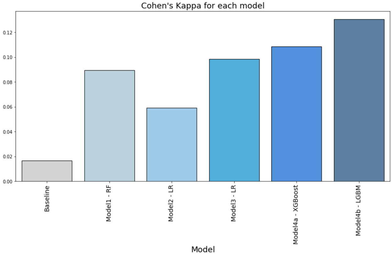
Cohen’s Kappa coefficient

Cohen’s Kappa is used to measure how well the model predictions perform relative to the actual outcomes. It is a statistic typically used to measure inter-rater reliability for qualitative items. It can be thought of as the proportionate agreement of a model predictions with actual results over the expected probabilities of agreement. Figure 1 below shows the Cohen’s Kappa measures for each model. Our models perform better than baseline. Model Strategy 4a using XGBoost and Model Strategy 4b using Light GBM are the best performing classifiers with Cohen’s Kappa greater than 10%.

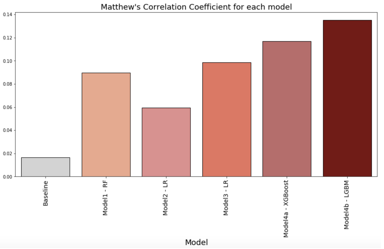
Matthew’s Correlation Coefficient

Similar to Cohen’s Kappa, Matthew’s Correlation Coefficient (MCC) is a balanced measure of how well a model predicts True Positives and True Negatives, which is useful in this case when the classes (decided and conflicted voter groups) are of different sizes. The MCC is a correlation coefficient between the observed and predicted binary classifications, returning a value between −1 and +1. A coefficient of +1 represents a perfect prediction, 0 no better than random prediction and −1 indicates total disagreement between prediction and observation. Figure 2 below shows the MCC measures for each model. Our models perform better than baseline. Model Strategy 4a using XGBoost and Model Strategy 4b using Light GBM are the best performing classifiers with MCC greater than 10%.

Precision

Model precision is an important evaluation metric given the cost of calling. Higher precision signals a higher rate of undecided voters correctly identified. This would mean minimizing false positives or when the model directs the caller to contact a decided voter instead of an undecided voter. Figure 3 shows the model precision metric for each model. All models perform better than baseline. Model precision is consistently above 40% for all models. Model Strategy 4a using XGBoost and Model Strategy 4b using Light GBM are the best performing classifiers with 50% precision.

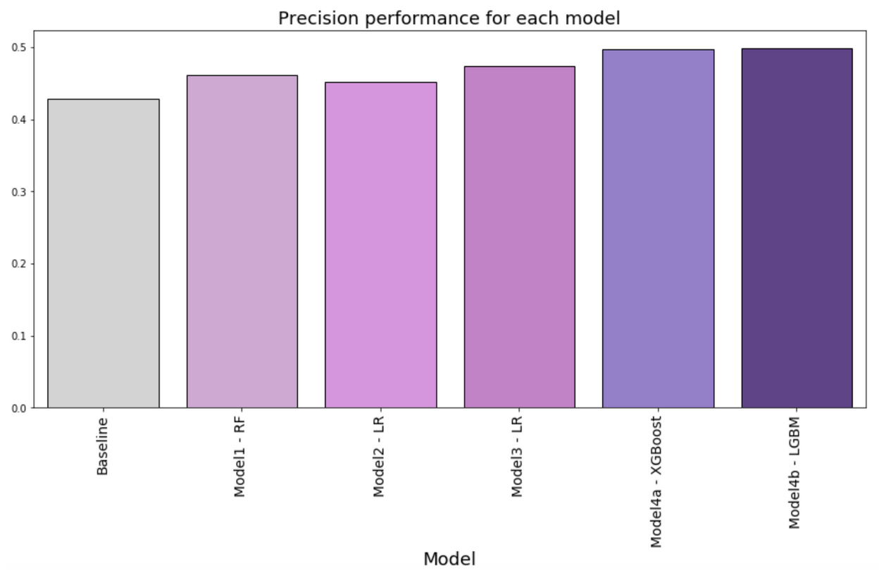
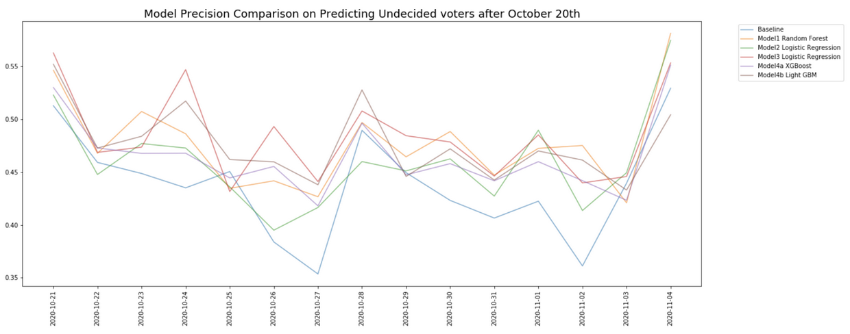
Figure 4 shows the model precision performance over time post-October 20th. We observe that no model consistently outperforms the others. While most models outperform the baseline model, there is no clear better model over all days. For example, we observe Model Strategy 3 with Logistic Regression implementation outperforms other models on October 24th, followed by a sharp underperformance on October 25th. We attribute this to the target voters being an elusive group. While, target voters might have certain persistent traits, shifts in the political climate and top-of-mind issues can lead to different sources of hesitancy on any given day particularly on days closer to the election.

Recall

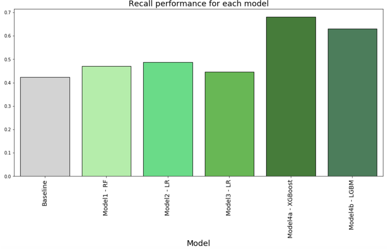
Model recall is an important evaluation metric given that failing to call actual undecided voters because the model considers them to be decided voters is an acute missed opportunity. This is particularly important in the context of competitive elections where even a small margin of votes may matter and failing to contact enough undecided voters could be consequential. Figure 5 shows the recall metric for each model. All models perform better than baseline. Model recall is consistently above 40% for all models. Model Strategy 4a using XGBoost and Model Strategy 4b using Light GBM are the best performing classifiers with recall above 60%. In particular Model Strategy 4a using XGBoost achieves 68% recall, while baseline is 42%.

Error Analysis

Confusion Matrix

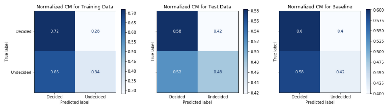
An analysis of the confusion matrix outcomes from binary classification predictions of decided versus undecided voters gives an understanding model performance. Figure 6 below is an example confusion matrix for the case problem.

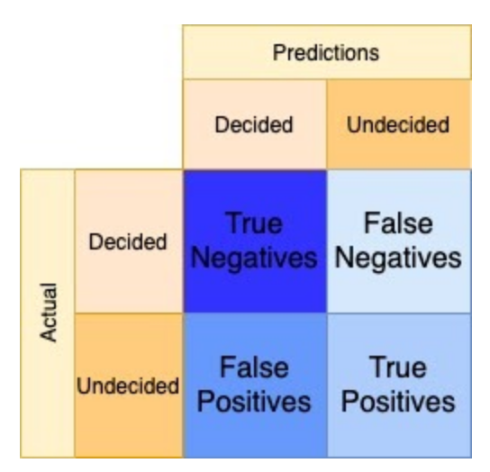
This view allows us to understand the negative predictive value, NPV, across the top row and positive predictive value, PPV or precision, across the bottom row.

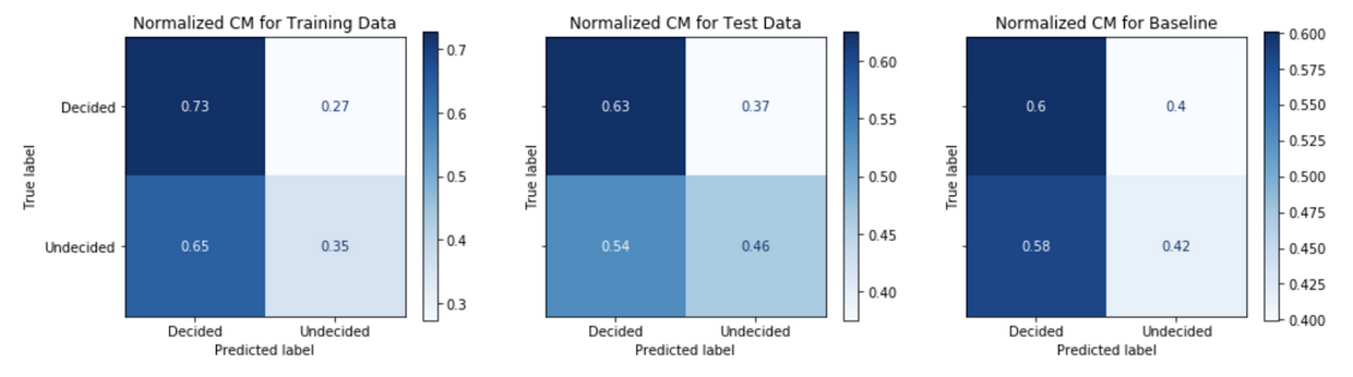
\[PPV = \frac{True\>positives}{True\>positives + False\>positives}\] \[NPV = \frac{True\>negatives}{True\>negatives + False\>negatives}\]

Comparing the confusion matrix performance on the train data to the performance on the test data (post-October 20th) tells us how well the model generalizes or fits to real data in the wild. A model that performs well on the train data, but performs poorly on the test date is said to overfit; whereas a model that performs poorly on the train data is said to be underfit. A comparison of the model’s performance on test data to the baseline model’s performance gives an informative evaluation measure of true performance. Figures 7-11 show the confusion matrix performance for each of the models.

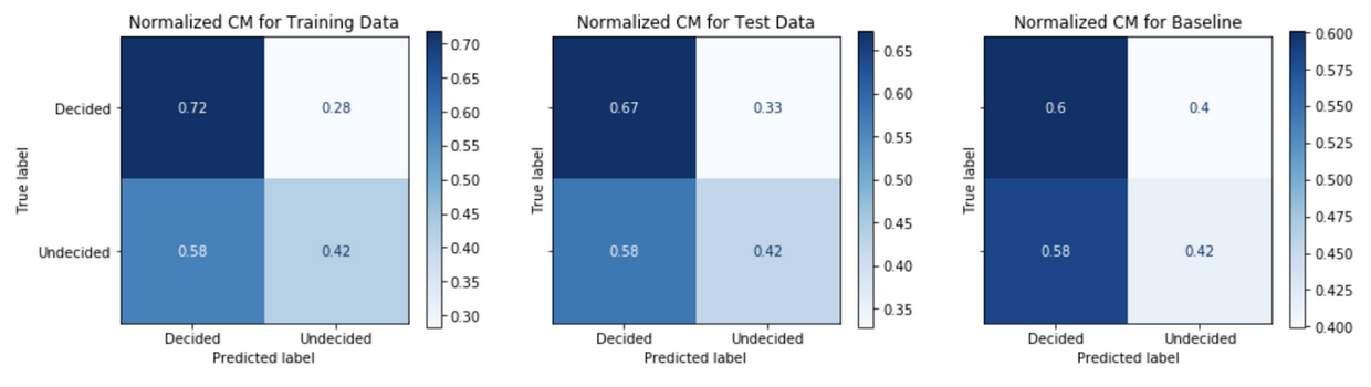
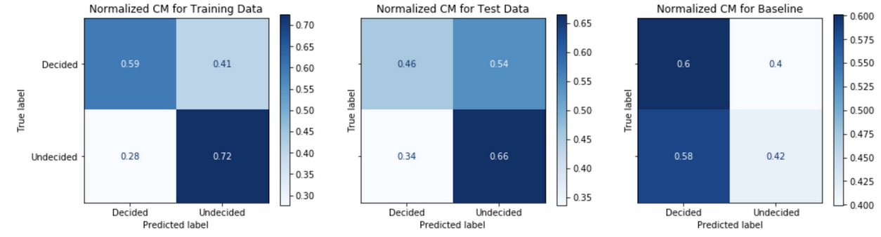
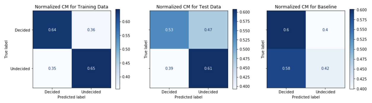
Generally, models have higher PPV in the test data as compared to the baseline model. The Model Strategy 4a and Model Strategy 4b implementations notably show much higher PPV in the test data as compared to the baseline model.

The Model Strategy 1 and Model Strategy 2 implementation generalizes well with an improvement in PPV going from the training data to the test data. The other models tend to generalize less well with mostly lower PPV going from training data to test data; however, the level of PPVs on the training data tends to be higher to begin with for the Model Strategies 4 and 5 implementations.

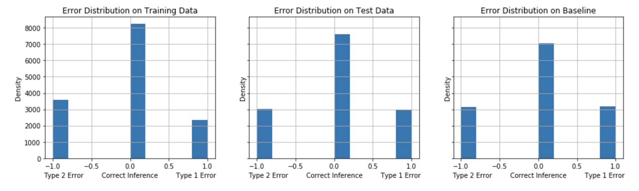
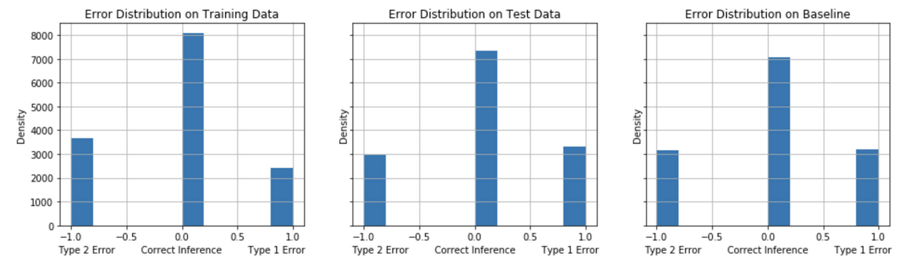
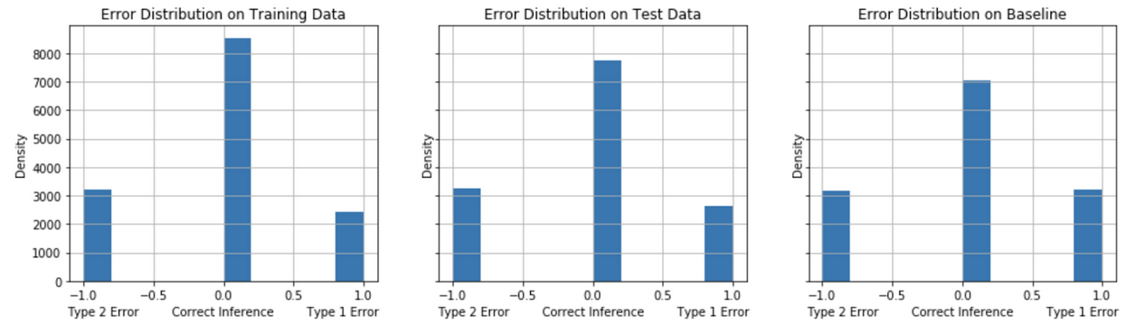
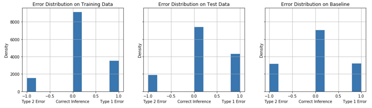
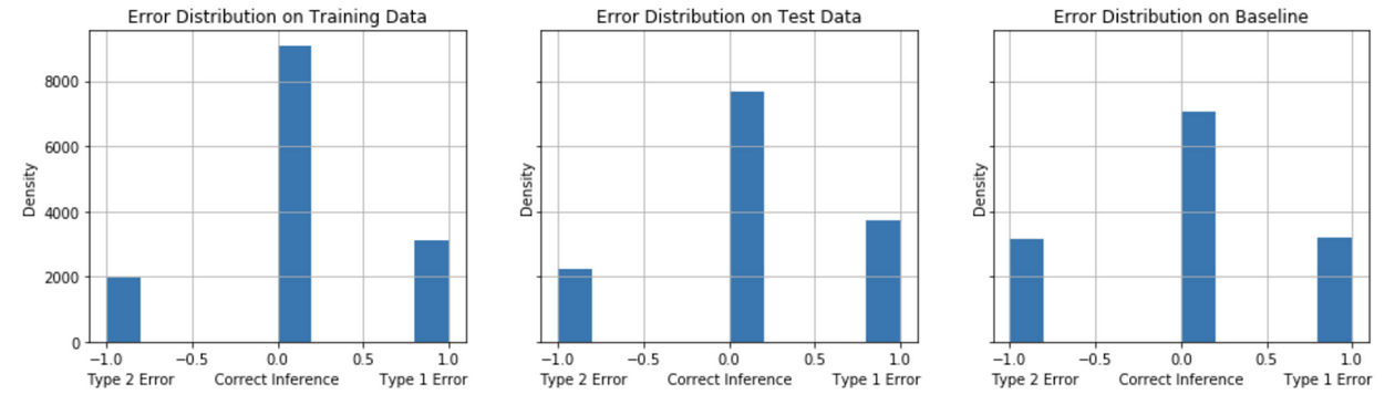
Balancing False Positives and False Negatives

The models are evaluated on their error distribution balance of Type 1 (False Positives) and Type 2 (False Negatives). For the problem of identifying undecided voters for a calling campaign in competitive election (“swing”) states, we seek to identify the model that, on balance, achieves a minimum of False Negatives and False Positives with a preference in minimizing False Negatives. A comparison of the models’ error distribution performance on test data to the baseline model’s performance gives an informative evaluation measure of true performance. Figures 12-16 show the error distribution for each of the models.

False Positives tend to decrease comparing the test performance to the baseline model performance for the Model Strategies 1, 2 and 3 implementations. The test performance of Model Strategies 4 and 5 implementations show a sharper decline in False Negatives with a somewhat small increase in False Positives compared to baseline.